PRIME (Polycomb Regulatory targets Integrated from Multi-source Evidence) is a freely accessible database and web resource for exploring candidate Polycomb group (PcG) target genes across human and mouse tissues, disease contexts and evidence types. PRIME integrates H3K27me3 ChIP-seq chromatin-state evidence, PcG perturbation RNA-seq functional-response evidence, curated literature records and external annotation resources to support context-resolved Polycomb target prioritisation.

COMPASS/PRIME framework overview

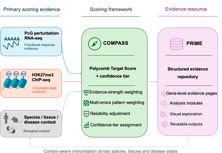
This overview shows how scoring evidence and biological context are integrated by COMPASS to generate a Polycomb Target Score (PTS) and confidence tier, which are then organised in PRIME as structured, searchable and reusable evidence records.

PRIME platform overview

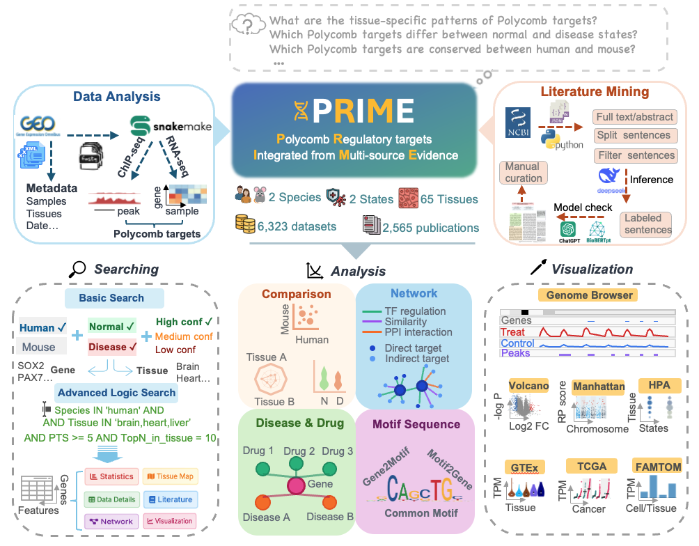
This overview shows how PRIME supports searching, browsing, evidence inspection, analysis modules, visual exploration and data download through a web-accessible database interface.

• PcG-focused evidence integration: PRIME combines H3K27me3 ChIP-seq evidence with PcG perturbation RNA-seq evidence. The current release includes 5,905 H3K27me3 ChIP-seq entries and 418 RNA-seq entries, together with 5,381 literature-derived associations and external resources including GTEx, TCGA, HPA and FANTOM5. These records cover human and mouse contexts across normal and disease states.
• Interpretable target prioritisation: COMPASS assigns each gene-context record a continuous Polycomb Target Score (PTS) and confidence tier using chromatin evidence, perturbation response, evidence convergence and context-specific reliability. PTS should be interpreted as a prioritisation score based on available evidence, not as direct proof of PcG-mediated repression at an individual locus.
• Evidence traceability and reusable outputs: PRIME provides gene search, category search, advanced search, dataset browsing, gene-level evidence pages, cross-context comparison, regulatory-network exploration, disease-drug annotation views, motif analysis, genome-browser visualisation and downloadable analysis-ready tables.

PRIME supports three search methods to find candidate Polycomb target records:

1. Category Search

Search by tissue, status, species, and confidence level:

• Species: Select Human or Mouse
• Tissue Types: Choose one or multiple tissues (default: all tissues)
• Sample Status: Filter by normal or disease status (multi-select supported)
• Confidence Level: Set to High, Medium, or Low (multi-select supported)
• Execute: Click Search to display filtered results

2. Gene Search

Search by gene names:

• Species: Select Human or Mouse (radio button selection)
• Status: Filter by Normal and/or Disease samples (checkbox selection)
• Confidence Level: Choose High, Medium, and/or Low confidence results (checkbox selection)
• Gene Names: Enter gene symbols in the text area (Click "Load Example Data" for quick testing with sample gene lists)

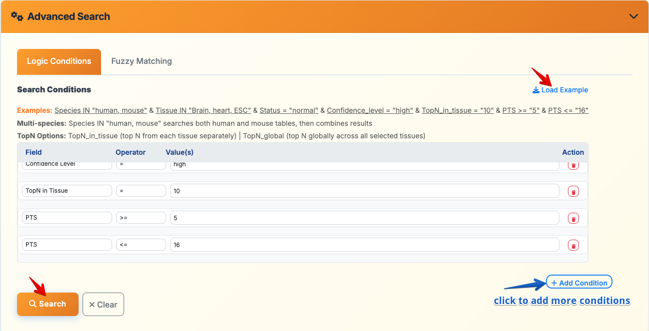
3. Advanced Search

Logic Conditions Mode:

• Flexible Query Builder: Add multiple search conditions using field-operator-value combinations
• Supported Fields: Species, Tissue, Status, Confidence Level, TopN settings, PTS values, etc.
• Multi-species Support: Search across human and mouse databases simultaneously
• TopN Options:
• TopN_in_tissue: Top N results from each tissue separately
• TopN_global: Top N results globally across all selected tissues
• Example Query: Species IN "human, mouse" & Tissue IN "Brain, heart, ESC" & Status = "normal" & Confidence_level = "high"

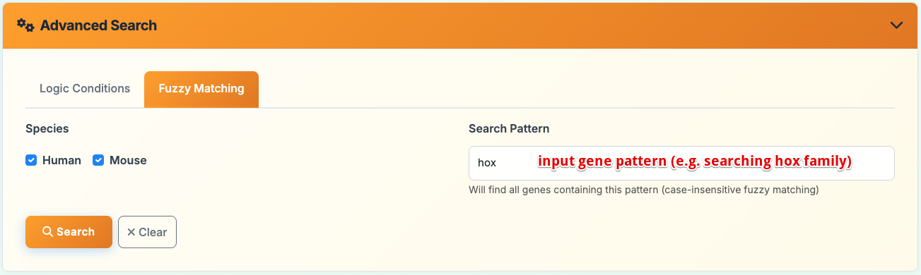
Fuzzy Matching Mode:

• Species Selection: Choose Human and/or Mouse (checkbox selection)
• Pattern Search: Enter gene name patterns for case-insensitive fuzzy matching
• Search Examples: hox, pax, sox (finds all genes containing these patterns)
• Flexible Matching: Identifies genes with partial name matches across selected species

Search Results (Data Page)

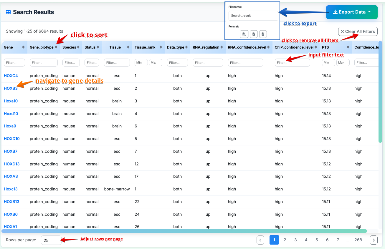
Data Table Columns:

• Gene: Gene symbol (e.g., HOXC4, HOXB3, Hoxa10)
• Gene_biotype: Gene classification (e.g. protein_coding, lncRNA)
• Species: Human or Mouse
• Status: Sample condition (normal/disease)
• Tissue: Tissue type (esc, brain, bone-marrow)
• Tissue_rank: Ranking within tissue
• Data_type: Evidence type (RNA-seq, ChIP-seq or both)
• RNA_regulation: Expression direction (up/down)
• RNA_confidence_level: RNA-seq evidence confidence (high/medium/low)
• ChIP_confidence_level: ChIP-seq evidence confidence (high/medium/low)
• PTS: Polycomb Target Score, an evidence-based prioritisation score (e.g., 15, 10)
• Confidence_level: Overall confidence rating (high/medium/low)

Interactive Features:

• Column Filtering: Each column has individual filter options
• Clear All Filters: Reset all applied filters
• Sortable Columns: Click column headers to sort data
• Customizable Display: Adjust rows per page (25 shown)
• Gene Hyperlinks: Click gene symbols to navigate to detailed gene information pages

Search Results (Gene Details Page)

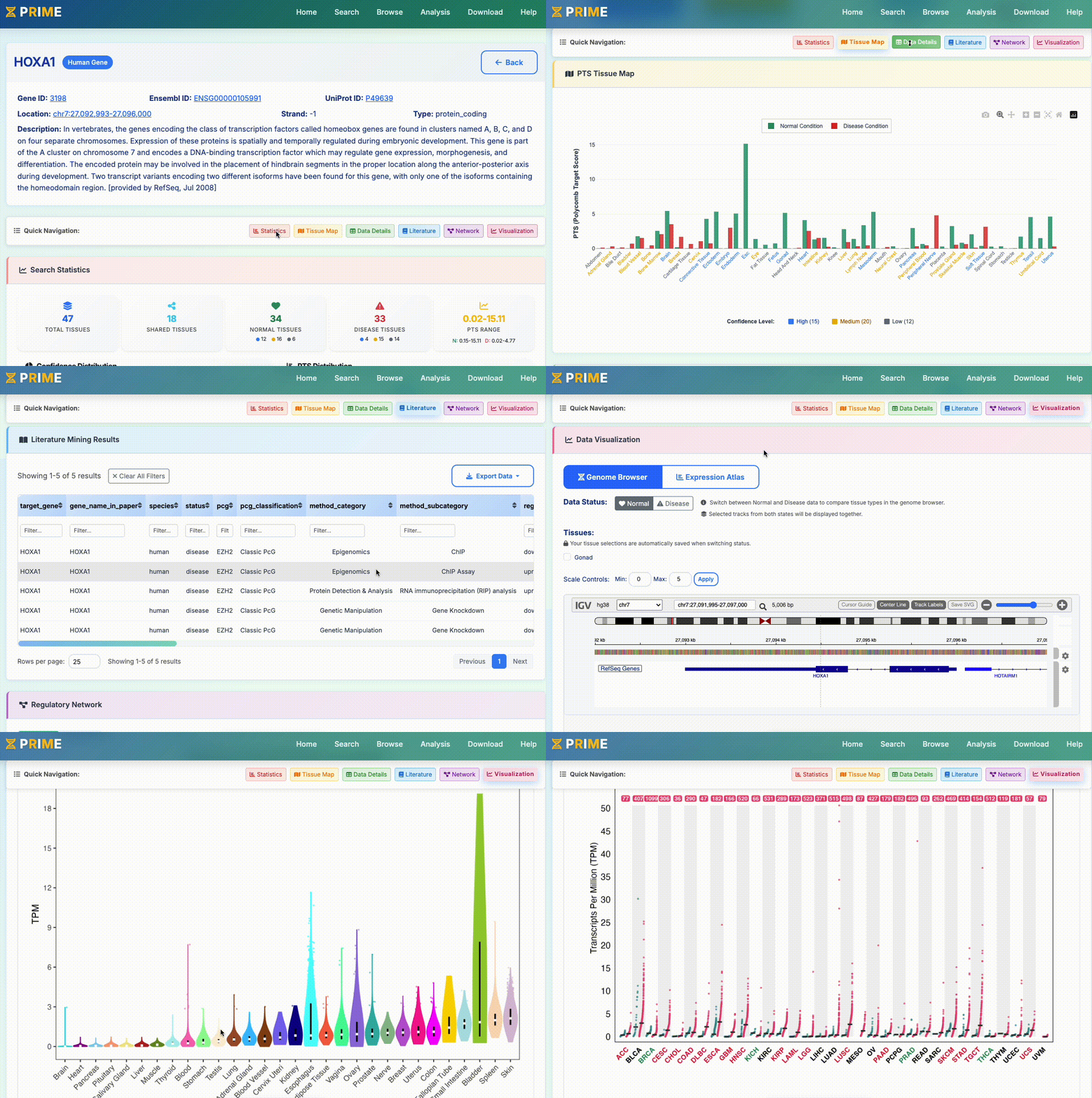
Users can search for genes from the home page or click on any gene name in the results table to access a gene-level evidence page. The page separates basic gene information, COMPASS-derived evidence, literature records, annotation layers and visualisation outputs so that users can inspect why a gene was prioritised.

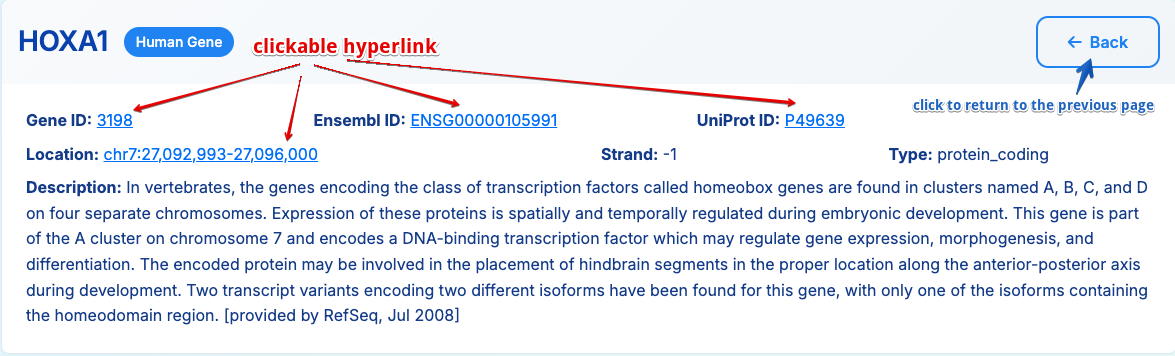
1. Gene Information

Basic gene details including: - Gene symbol, NCBI gene ID, Ensembl ID, UniProt ID and genomic location - External database links (GeneCards, NCBI, Ensembl, UniProt and UCSC DNA sequence)

• Strand orientation and gene type
• NCBI gene functional summary

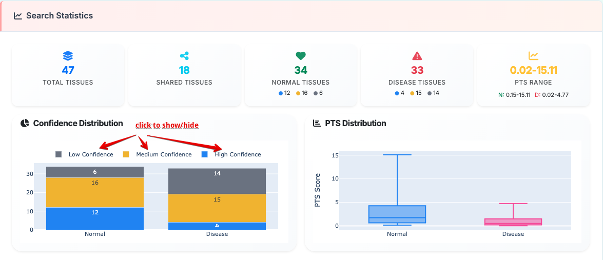
2. Search Statistics

Comprehensive database analytics providing:

• Tissue coverage metrics across normal and disease conditions
• Confidence distribution analysis with quality assessment indicators
• PTS score comparison between sample types

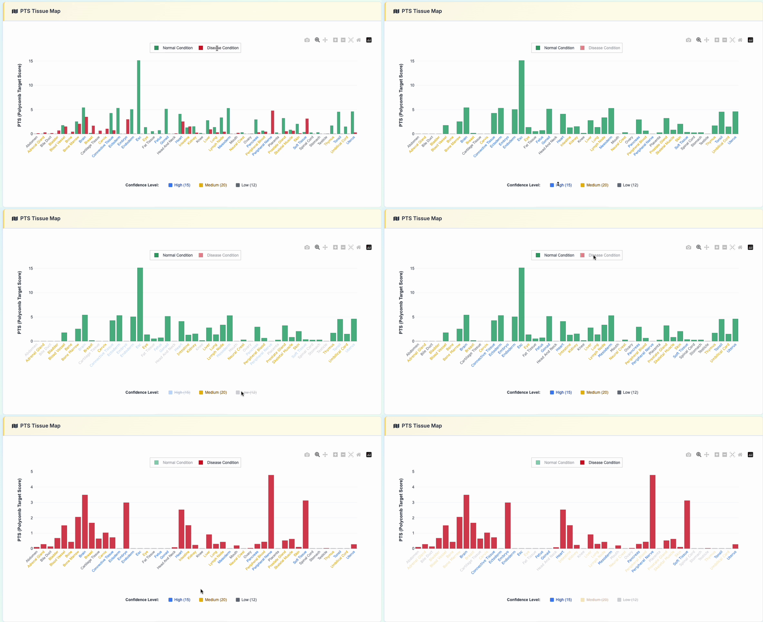
3. PTS Tissue Map

Interactive Polycomb target-prioritisation view featuring: - Comparative PTS profiles across tissue types - Normal vs Disease condition toggle display - Interactive legend controls for selective data viewing

Click the "show details" button to reveal the specific data used：

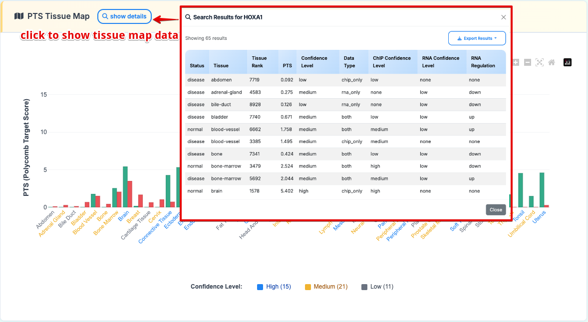
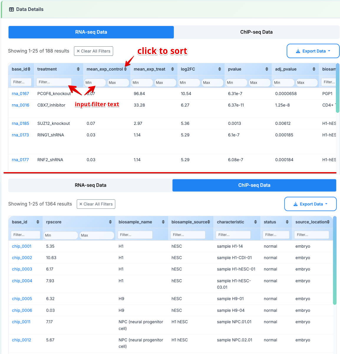
4. Data Details

• base_id ：Unique dataset identifier for traceability

• biosample_name: Experimental cell/tissue type (e.g., H1-hESC, CD4+ T cells)

• status: Sample classification (normal vs. disease states)

• characteristic: Specific experimental conditions or sample annotations

RNA-seq Data Key Columns：

• treatment: Experimental perturbation targeting Polycomb group proteins

• mean_exp_control: Baseline expression level in control conditions

• mean_exp_treat: Expression level following experimental treatment

ChIP-seq Data Key Columns：

• rpscore: Regulatory Potential Score (Higher scores indicate stronger H3K27me3 regulatory potential)

5. Literature Mining

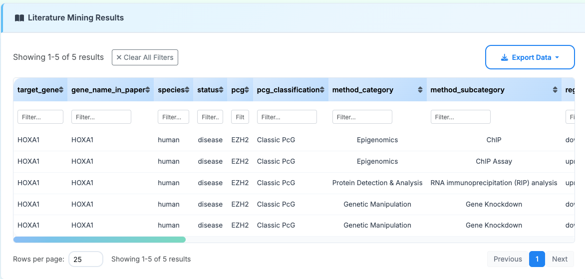
Literature-derived records provide curated context for reported PcG-gene relationships. These records are displayed as supporting annotations and are not used to calculate or update PTS.

Key columns include:

• target_gene: Standardised gene symbol mapped to PRIME gene records
• Represents a gene reported in the literature in relation to PcG regulation or PcG-associated evidence
• gene_name_in_paper: Gene name as written in the original publication
• May differ from the standardised symbol because of synonyms, aliases or naming conventions
• pcg: Polycomb component, complex or related term reported in the source text
• Examples: BMI1, SUZ12, EZH2, CBX7, PRC1, PRC2, PcG, H3K27me3
• pcg_classification: Functional classification of the Polycomb-related term
• Classic PcG: Core Polycomb repressive-complex components with established chromatin regulatory roles
• Non-classic PcG: Auxiliary or Polycomb-associated factors with emerging or context-dependent roles
• General term: Broad concepts referring to Polycomb complexes, histone marks or collective PcG activity
• method_category: Broad experimental approach used in the source study
• Examples: Genetic manipulation, ChIP-seq, expression analysis
• method_subcategory: Specific experimental technique within the broader category
• Examples: Gene knockdown, gene knockout, overexpression
• regulation: Reported expression or regulatory direction where available
• Examples: upregulated, downregulated, no change

Literature records help users trace published support, but they should be interpreted together with COMPASS-derived RNA-seq and H3K27me3 evidence.

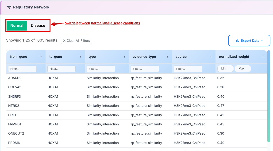
6. Regulatory Network

The regulatory-network section displays interaction and annotation links connected to the selected gene. These links are useful for evidence inspection and hypothesis generation, but they should not be interpreted as proof of direct regulation.

Gene interaction network columns include:

• from_gene: Source gene in the displayed interaction or annotation link
• to_gene: Target gene or interaction partner
• type: Category of molecular or evidence relationship
• Similarity_interaction: Similarity based on H3K27me3 regulatory-potential features
• PPI_interaction: Protein-protein interaction evidence
• PcG_regulation: PcG-related regulatory evidence from PRIME records or literature-derived annotations
• TF_regulation: Transcription-factor regulatory relationship from external resources
• evidence_type: Evidence source or support level
• Examples: rp_feature_similarity, protein_interaction, high_confidence_regulation, medium_confidence_regulation, low_confidence_regulation, text_mining, molecular_interaction_assay
• source: Database or experimental origin of the link
• Examples: H3K27me3_ChIPseq, STRING_database, Knock_PcG_RNAseq, TRRUST, TFLink, GTRD, ReMap
• weight_normalized: Normalised evidence weight used for visual ranking in the network
• Higher values indicate stronger support within the displayed network, not direct proof of mechanism

7. Data Visualization

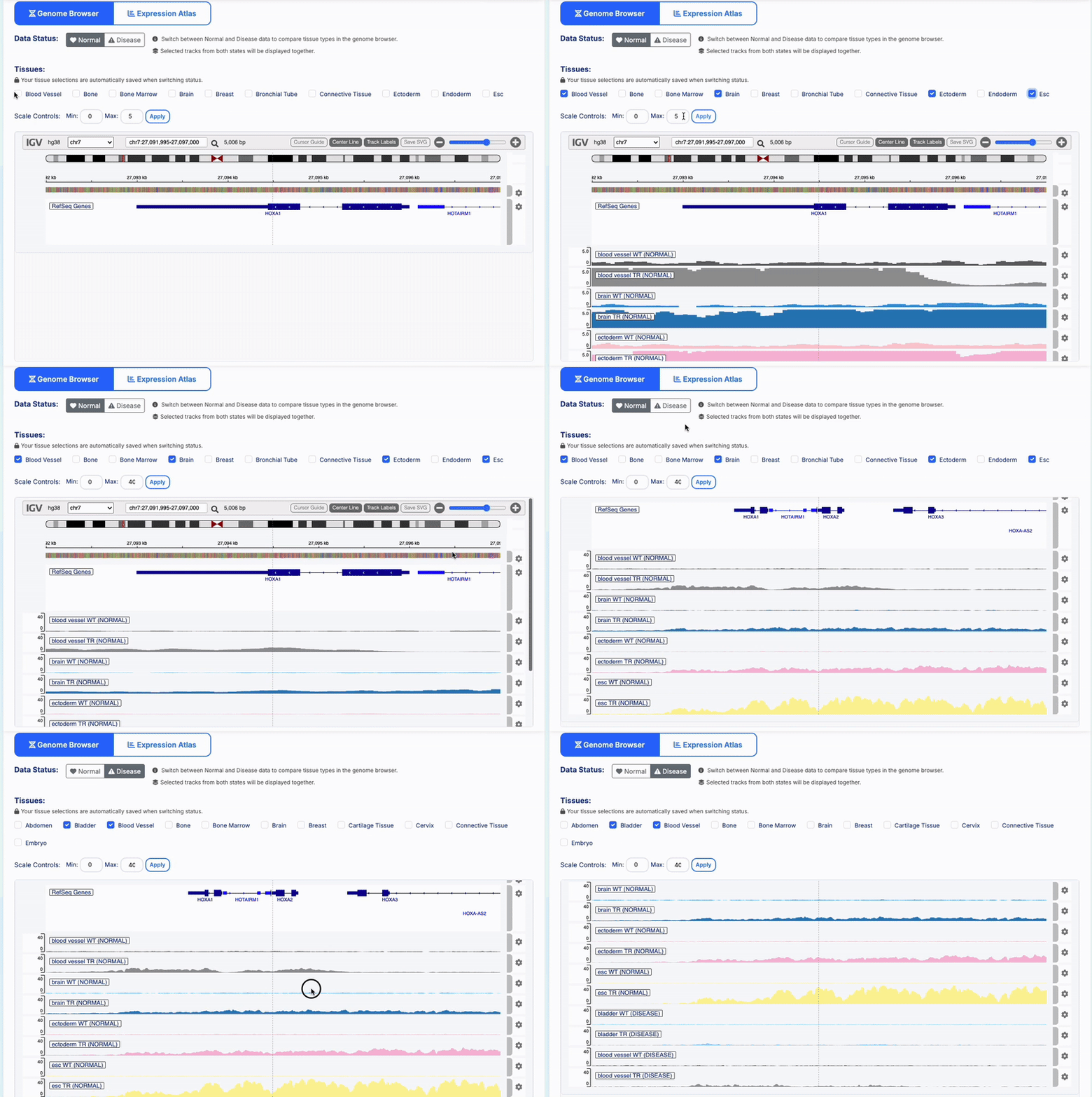
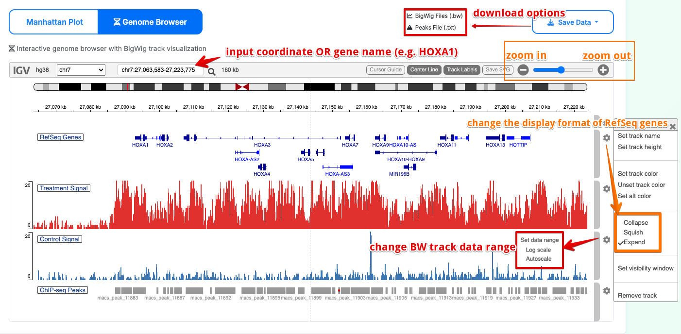
Interactive Genome Browser

• Multi-tissue Support: Select from 30+ human tissues and 20+ mouse tissues
• Dynamic Loading: Tissue options update automatically based on species and data availability

• State Preservation: Tissue selections are automatically saved when switching between Normal/Disease status

• Manual Scale Setting: Adjust Min and Max values to normalize all loaded tracks to the same scale range

• RefSeq Annotations: Gene structure display with exon/intron boundaries

• Interactive Navigation: Search genes, zoom regions, and explore genomic context
• Track Management: Color-coded tissue-specific tracks with WT/TR treatment indicators

Expression Atlas

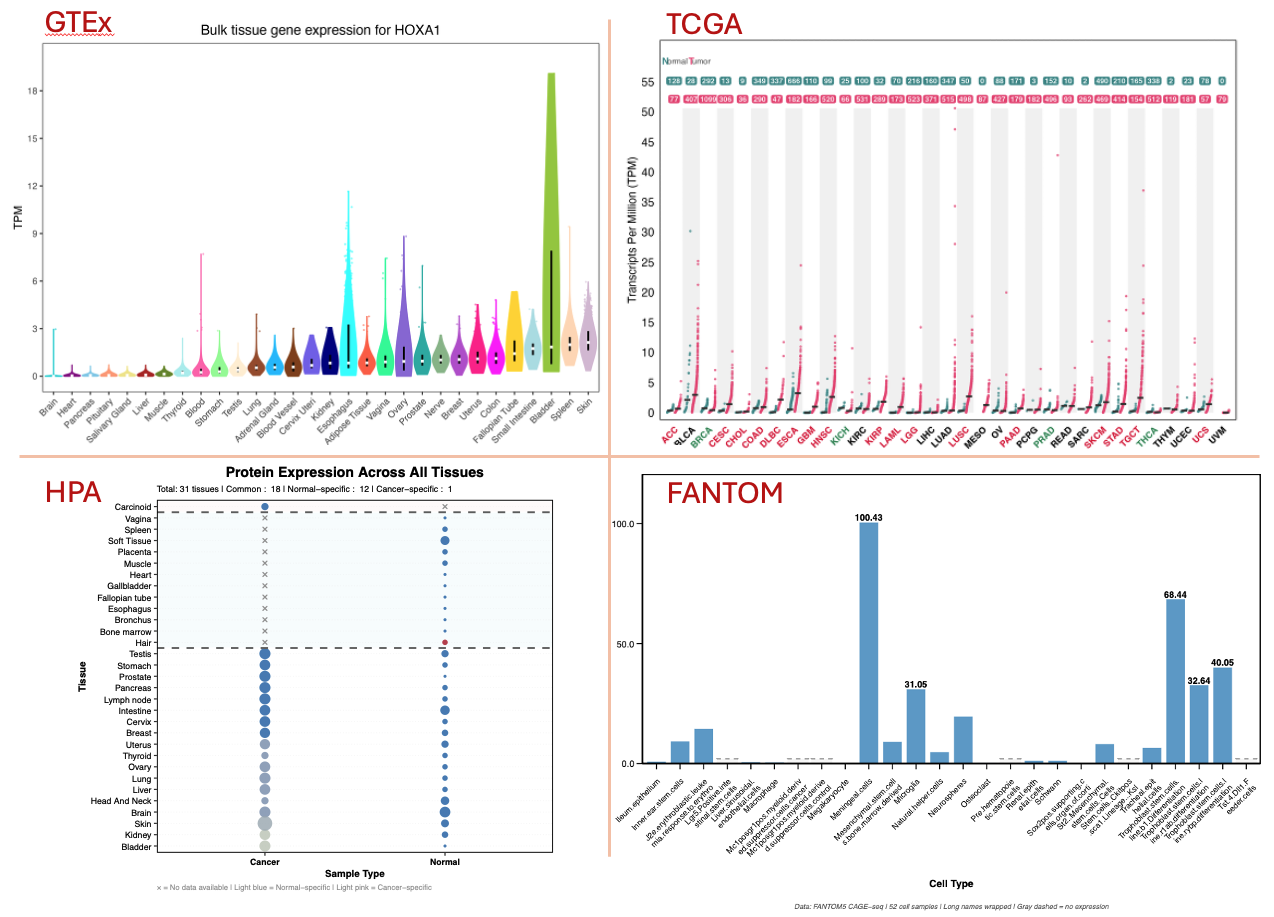
[Note: some genes may not have data available in this database, resulting in no image results]

• GTEx (Genotype-Tissue Expression)
• Normal tissue expression across 30+ human tissues
• Violin plots showing expression distribution and median values

• Tissue-specific color schemes for visual clarity

• TCGA Pancancer (The Cancer Genome Atlas)

• Cancer tissue expression data across multiple tumor types
• Dot plots comparing normal vs tumor expression levels

• Disease-associated expression context for interpretation

• Human Protein Atlas (HPA)

• Protein-level expression data across human tissues
• Immunohistochemistry and proteomics-based measurements

• Tissue specificity and subcellular localization information

• FANTOM5 (Functional Annotation of the Mammalian Genome)

• Mouse tissue and cell-type specific expression
• Two data types: tissue_level and cell_level analysis
• Dual-panel visualization due to extensive tissue coverage

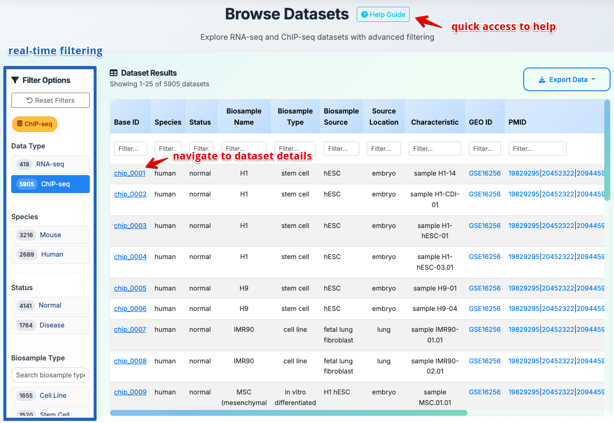
Browse curated RNA-seq and H3K27me3 ChIP-seq evidence entries with advanced filtering and interactive data exploration.

Filter Options

• Data Type: RNA-seq, ChIP-seq
• Species: Human, Mouse
• Tissue/Cell Type: Organ-specific datasets
• Experimental Conditions: Normal, Disease, Treatment (for RNA-seq)

Results Navigation

• Real-time Filtering: Click left panel options, table updates automatically
• Column Sorting: Click column headers for ascending/descending order
• Pagination: Display 10-250 rows per page
• Data Export: CSV, Excel, TXT formats

Browse Results

Upon selecting a Dataset ID from the browse results, the user will be directed to a comprehensive dataset analysis page, which is systematically organized into three primary sections:

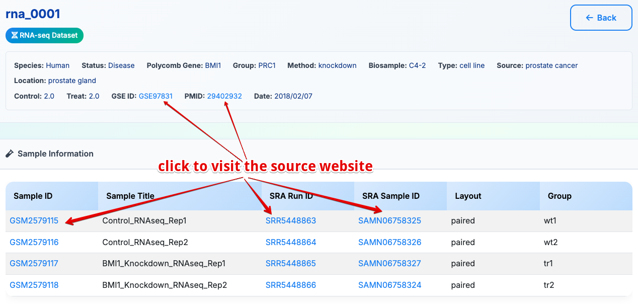
1. Sample Information

Dataset metadata and experimental details: - Sample ID and external database links - Experimental conditions and treatments - Data type classification (RNA-seq/ChIP-seq) - Publication information and PubMed links

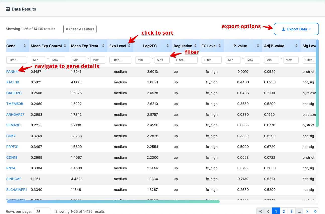
2. Data Details

• Gene: Gene symbol with a hyperlink to the gene details page

• Source_location: Tissue or cell type origin

• Status: Disease state (Normal, Disease)

RNA-seq Data Key Columns：

• Mean Exp Control: Mean expression level in control samples
• Mean Exp Treat: Mean expression level in treatment samples
• Exp Level: Expression category (High, Medium, Low)
• High exp: Above 75th percentile in control or treatment group
• Medium exp: Between 35th and 75th percentiles

• Low exp: Below 35th percentile in control or treatment group

• FC Level: log2 Fold change magnitude category (High FC, Medium FC, Low FC, No change)

• High FC: Above 75th percentile [Strong biological relevance]
• Medium FC: Above 50th percentile [e.g. log2FC ≈ 0.585 equals 1.5-fold change]
• Low FC: Above 25th percentile [e.g. log2FC ≈ 0.265 equals 1.2-fold change]

• No Change: Below all dynamic thresholds [Changes likely from technical noise]

• Sig Level: Statistical Significance Levels

• FDR Strict (fdr_strict): adj_pvalue < 0.01
• FDR Relaxed (fdr_relaxed): adj_pvalue < 0.05
• P-value Strict (p_strict): pvalue < 0.01 (when FDR unavailable)
• P-value Relaxed (p_relaxed): pvalue < 0.05 (when FDR unavailable)
• Not Significant (not_sig): Insufficient statistical evidence
• Confidence Level: Quickly assess data quality
• High Confidence: FDR < 0.01 AND High fold change AND High expression
• Medium Confidence: Strict significance (FDR/p < 0.01) AND Medium fold change or Standard significance (FDR/p < 0.05) AND Medium/High fold change
• Low Confidence: Any significance level AND Low fold change or Weak significance AND Medium fold change or Observable trend without statistical support

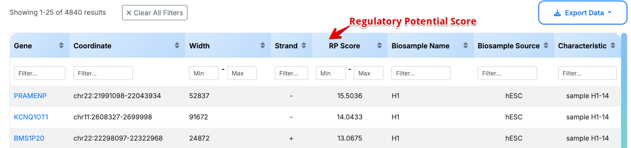
ChIP-seq Data Key Columns：

RP Score (Regulatory Potential Score): gene-level H3K27me3 regulatory-potential evidence derived from peak location and peak signal. Higher scores indicate stronger H3K27me3-associated chromatin evidence near or within the gene, not direct proof of PcG-mediated repression.

RP_Score = Σ(distance_score × peak_signal) / √(number_of_peaks)

• distance_score: Location-based weight assigned to each peak
• peak_signal: H3K27me3 ChIP-seq signal intensity at the peak
• √(number_of_peaks): Normalisation to reduce artificial inflation from genes with many peaks

Distance score calculation:

• Promoter region: distance_score = exp(-0.004 × |distance_to_TSS|)
• Peaks closer to the transcription start site receive higher weights
• Example: TSS (distance = 0) → score = 1.0; 500 bp away → score ≈ 0.135
• Intragenic region: distance_score = 0.4
• Moderate regulatory-potential weight for peaks located within the gene body
• Intergenic region: distance_score = 0.3
• Lower regulatory-potential weight for distal peaks

Example: For a gene with 3 H3K27me3 peaks:

Peak 1: Promoter, distance=500bp, signal=100
→ distance_score = exp(-0.004 × 500) = 0.135
→ contribution = 0.135 × 100 = 13.5

Peak 2: Intragenic, signal=80
→ distance_score = 0.4
→ contribution = 0.4 × 80 = 32.0

Peak 3: Intergenic, signal=60
→ distance_score = 0.3
→ contribution = 0.3 × 60 = 18.0

RP_Score = (13.5 + 32.0 + 18.0) / √3 = 63.5 / 1.73 = 36.7

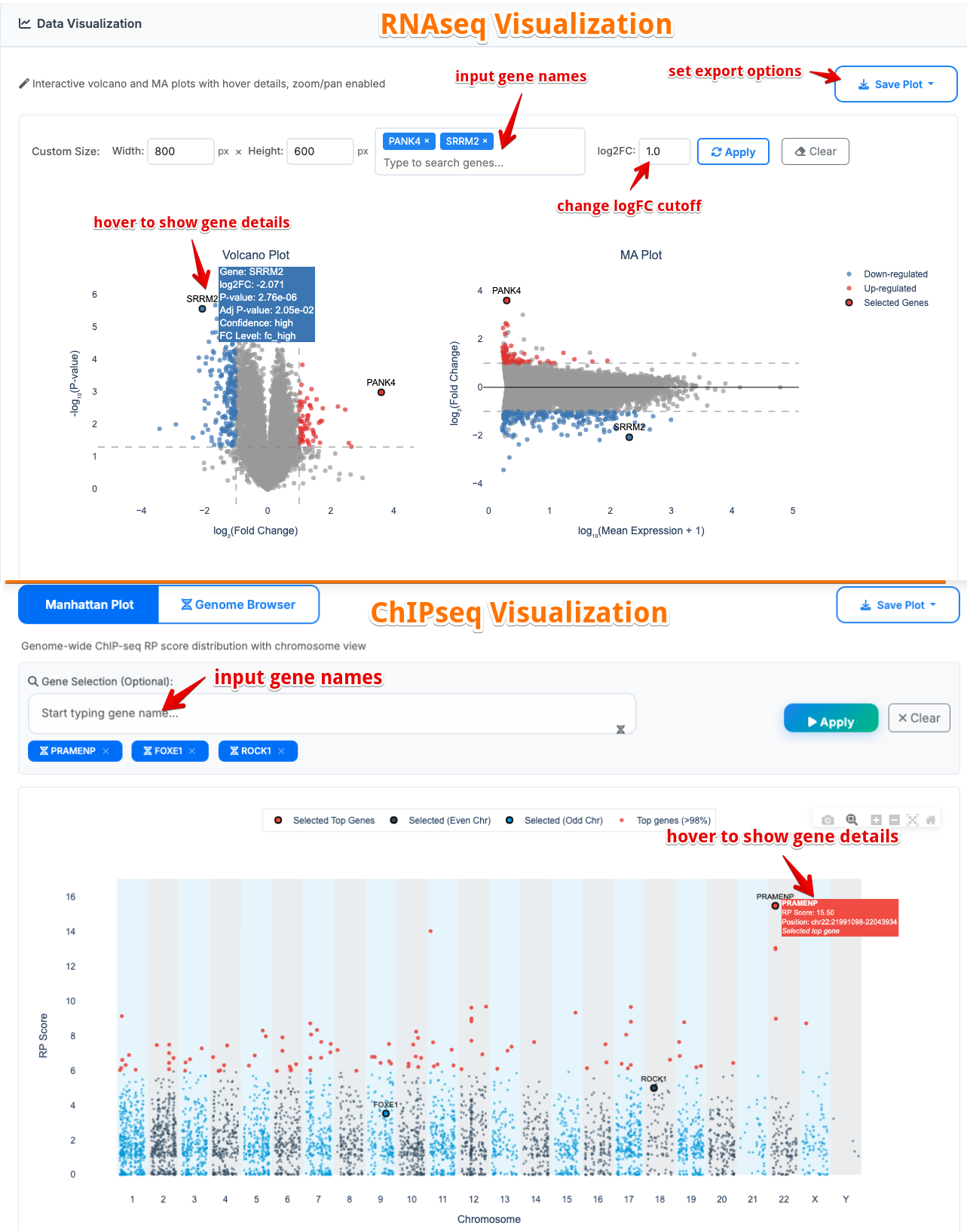
3. Data Visualization

Interactive plots showing dataset characteristics:

• Volcano Plot: Differential expression analysis
• MA Plot: Mean expression vs fold change
• Manhattan Plot: Genome-wide significance mapping
• Custom plot dimensions and export options (PNG/PDF/SVG/HTML)

Interactive genomic data visualization:

• Automatically load hg38 or mm10 according to the species of the ChIP-seq dataset
• Scale normalization and track management
• Real-time genomic region navigation
• Provide complete downloads for BW and peak files

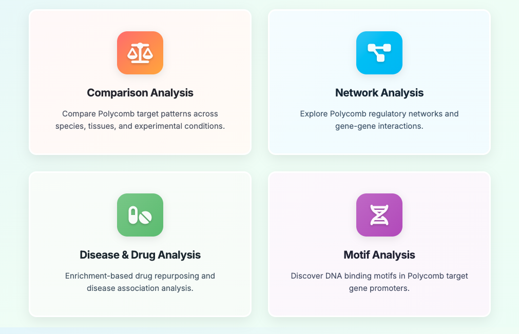
PRIME provides four analysis tools to explore candidate Polycomb target records and their downstream annotations. These modules use precomputed COMPASS outputs and annotation tables; they do not recalculate PTS or change confidence tiers.

Compare precomputed PTS profiles across species, tissues and sample status to inspect context-specific Polycomb target-prioritisation patterns.

Sub-Module 1: Species Comparison

Purpose: compare the same or comparable tissue between human and mouse to inspect cross-species target-set similarity and species-specific prioritisation patterns.

Usage:

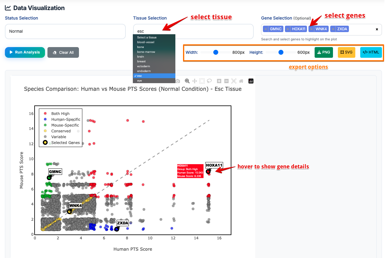
1. Select status: Choose normal or disease from the dropdown menu
2. Choose tissue: Select one tissue
3. Input gene name (optional): Enter one or more genes to display on the plot
4. Run Analysis: Click the button to generate dynamic plots
5. Download Results: Export volcano plots and MA plots in PNG/SVG/HTML formats
6. Clear All: Reset all parameters and clear the image

Scatter plot result:

• Both High (Red Points): human_score > 80th percentile AND mouse_score > 80th percentile
• Meaning: Genes with strong prioritisation evidence in both species
• Location: Upper right quadrant
• Human-Specific (Blue Points): human_score > 80th percentile AND mouse_score < 20th percentile
• Meaning: Higher prioritisation evidence in human than in mouse for the selected context
• Location: Lower right quadrant
• Mouse-Specific (Green Points): human_score < 20th percentile AND mouse_score > 80th percentile
• Meaning: Higher prioritisation evidence in mouse than in human for the selected context
• Location: Upper left quadrant
• Conserved/Similar (Yellow Points): |human_score - mouse_score| < 25th percentile of all differences
• Meaning: Similar PTS values between species in the selected context
• Location: Along the diagonal
• Variable (Gray Points): All other genes not fitting the categories above

This module provides descriptive cross-species comparison of precomputed PTS profiles. It should not be interpreted as direct conservation of repression strength.

Sub-Module 2: Tissue Comparison

Purpose: compare Polycomb Target Scores (PTS) across tissues within normal and disease status to inspect tissue-specific prioritisation patterns.

Usage:

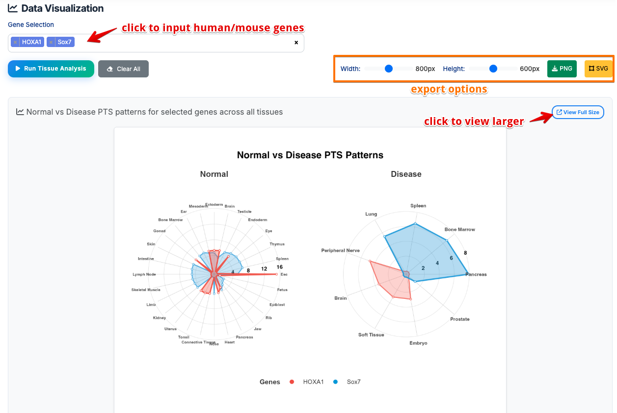
1. Input Gene Names: Enter one or more human/mouse gene symbols (e.g., HOXA1, Sox7)
2. Run Analysis: Click button to generate interactive radar charts
3. Download Results: Export radar plots in PNG/SVG formats

Radar Chart Results:

• Tissue-specific prioritisation: Sharp spikes in specific directions

• Meaning: Higher PTS in one or a few tissues

• Broad prioritisation pattern: Circular or symmetric polygon shape

• Meaning: Similar PTS across multiple tissues

Sub-Module 3: Status Comparison

Purpose: compare Polycomb Target Scores (PTS) between normal and disease conditions within tissues to inspect disease-associated shifts in target prioritisation.

Usage:

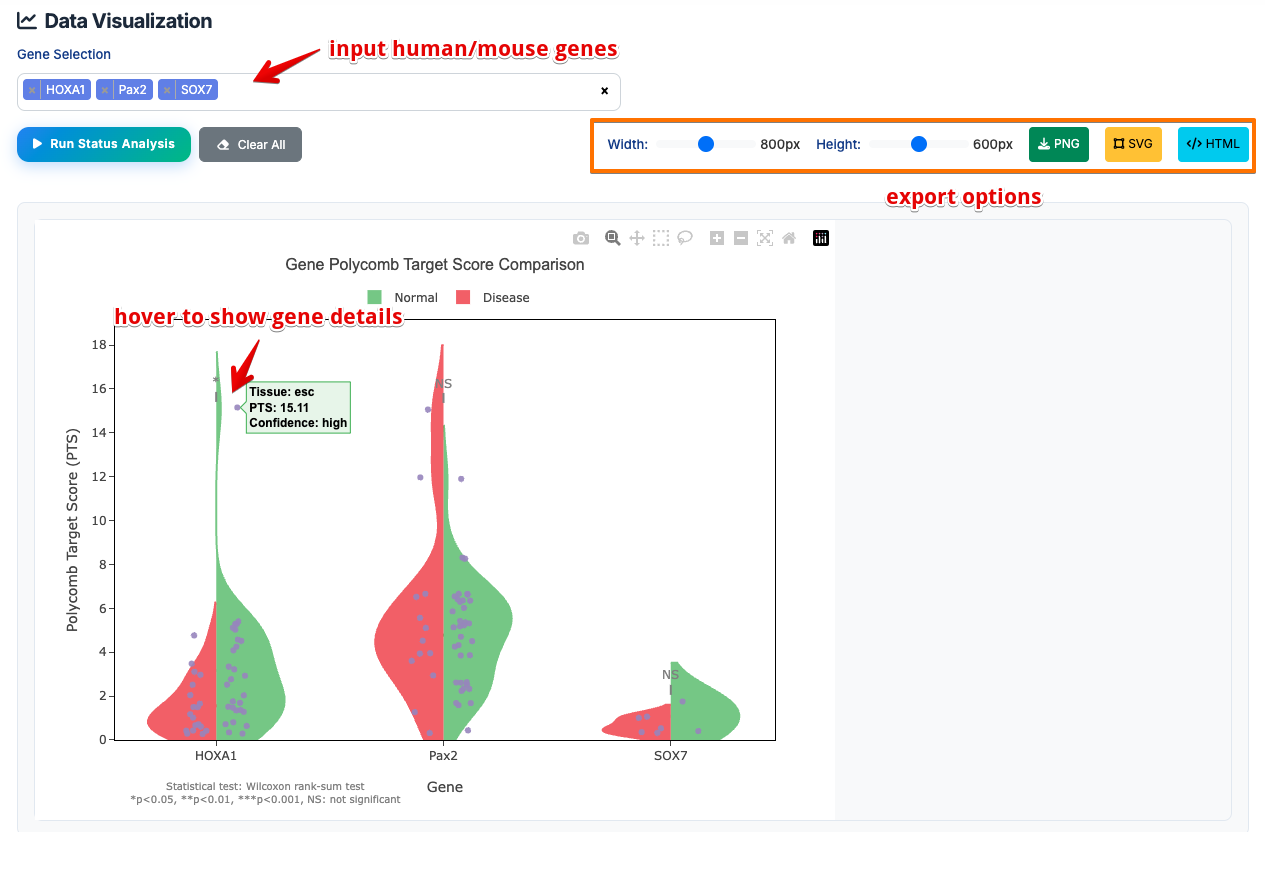
1. Input Gene Names: Enter one or more human/mouse gene symbols (e.g., HOXA1, Pax2, SOX7)
2. Run Analysis: Click button to generate interactive violin plots
3. Download Results: Export violin plots in PNG/SVG/HTML formats

Violin Plot Results:

• Normal Status (Right Side/Green): Shows PTS distribution in normal conditions
• Disease Status (Left Side/Red): Shows PTS distribution in disease conditions
• Each point represents the PTS value of a tissue, and users can hover to view the details.

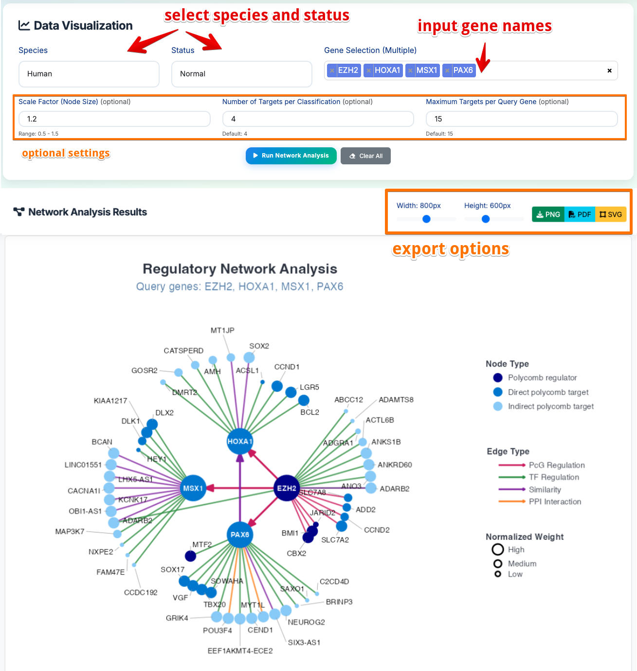
Purpose: Build evidence-based regulatory and interaction networks around selected genes. The network module helps users inspect hub-like genes, protein-protein interactions, PcG-related evidence links, transcription-factor links and similarity-based relationships. Network links are intended for exploration and hypothesis generation, not as proof of direct mechanism.

Usage:

1. Select Species: Choose Human or Mouse from the dropdown menu
2. Select Status: Choose Normal or Disease condition
3. Input Query Genes: Enter gene symbols of interest (e.g., EZH2, MSX1, HOXA1, PAX6)
4. Set Parameters: Adjust hub gene degree threshold and maximum targets per query
5. Run Analysis: Click the button to generate an interactive network diagram
6. Download Results: Export network plots in PNG/PDF/SVG formats

Network Visualization Results:

• Central Hub Genes (Large Dark Nodes): Highly connected genes in the displayed network
• Meaning: Genes with many evidence links or interaction partners in the selected query result
• Query Genes (Large Colored Nodes): User-specified genes of interest
• Meaning: Starting points for network exploration
• Connected Genes (Small Nodes): Candidate targets, regulators or interaction partners linked to query genes
• Meaning: Genes connected by PcG-related evidence, TF annotations, PPI records or similarity links
• Node Colors by Function:
• Dark Blue: PcG regulators or PcG-related components
• Medium Blue: Candidate PcG target records with stronger support
• Light Blue: Candidate PcG target records with weaker or indirect support
• Edge Colors by Interaction Type:
• Red: PcG-related evidence link (PcG_regulation)
• Green: Transcription-factor annotation (TF_regulation)
• Purple: Similarity pattern (Similarity_interaction)
• Orange: Protein-protein interaction (PPI_interaction)
• Node Size: Represents normalised network evidence weight
• Circle size supports visual ranking within the displayed network and should not be interpreted as causal strength

Purpose: Explore disease and drug annotation layers linked to candidate Polycomb target records. This module combines disease annotations and drug-gene records to help prioritise follow-up questions. The outputs are annotation-based hypotheses and should not be interpreted as therapeutic recommendations or proof that a gene drives a disease mechanism.

Usage:

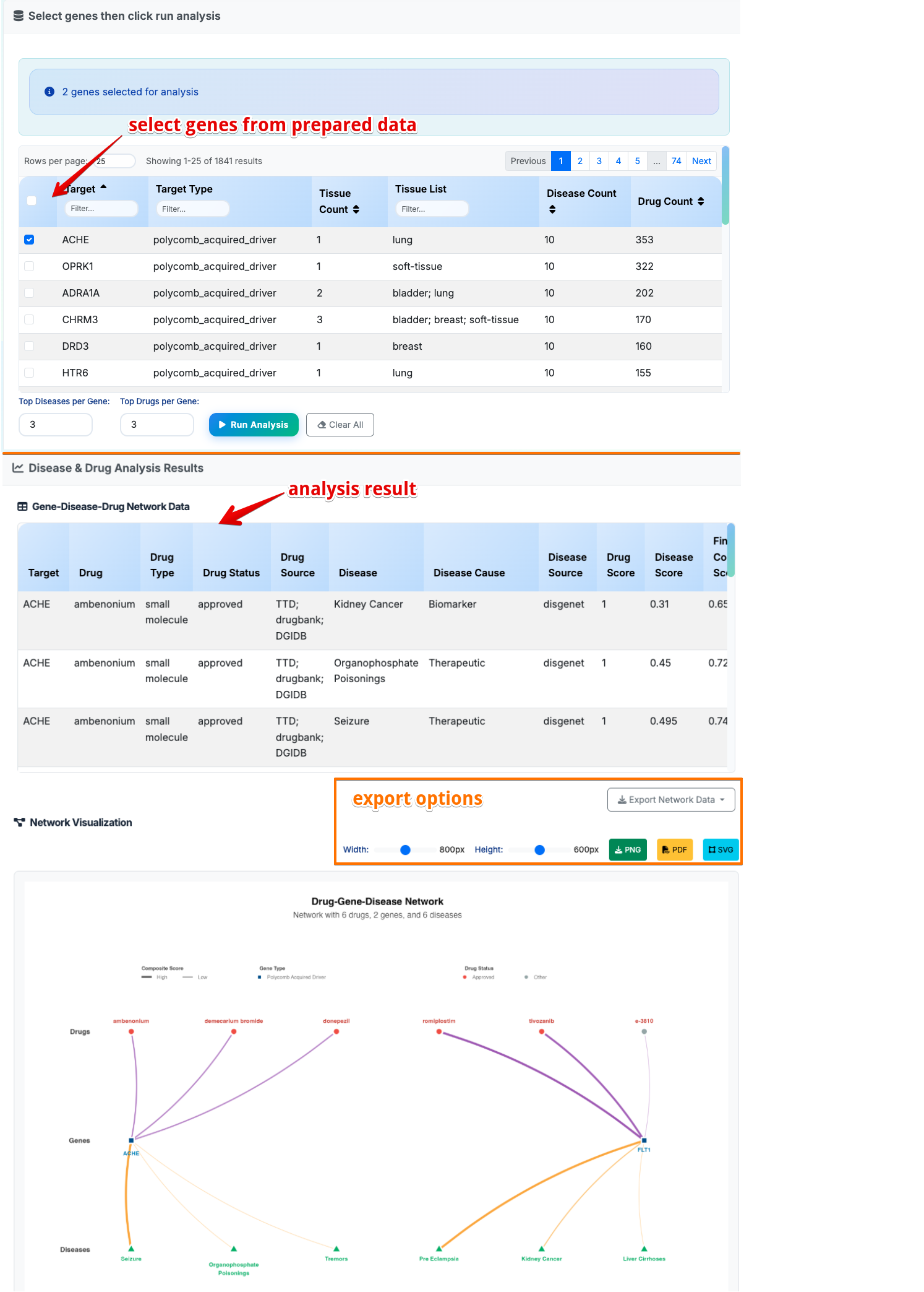
1. Browse Gene Targets: The interface loads candidate Polycomb target records with disease annotations
2. Target Type:
   • Polycomb-acquired candidates: genes showing stronger Polycomb-associated prioritisation in disease-context records than in matched or comparable normal contexts
   • Polycomb-perturbed biomarkers: genes whose Polycomb-associated evidence profile changes in disease-context records and may be useful for follow-up investigation
3. Tissue Count: Number of tissues or contexts where the target has evidence
4. Tissue List: Specific tissues or contexts with Polycomb-associated evidence
5. Disease Count: Number of linked disease annotations
6. Drug Count: Number of linked drug-gene records
7. Select Genes: Use table filtering and checkboxes to select genes of interest
8. Set Parameters: Adjust top diseases per gene and top drugs per gene
9. Run Analysis: Click the button to generate results

Gene-Disease-Drug Network Data Results:

• Target: Selected candidate Polycomb target gene
• Drug: Drug or compound linked to the gene in external drug-gene resources
• Drug Type: Classification of drug mechanism or interaction type where available
• Drug Status: Development stage (e.g., approved, investigational, experimental)
• Drug Source: Database source of drug information (e.g., TTD, DrugBank, DGIdb)
• Disease: Associated disease name
• Disease Cause: Disease-annotation category where available (e.g., mutation, biomarker)
• Disease Source: Database source of disease association (e.g., DisGeNET, Orphanet)
• Drug Score: Computational or database-derived drug-target annotation score
• Disease Score: Gene-disease association score
• Final Composite Score: Integrated annotation score for ranking follow-up candidates
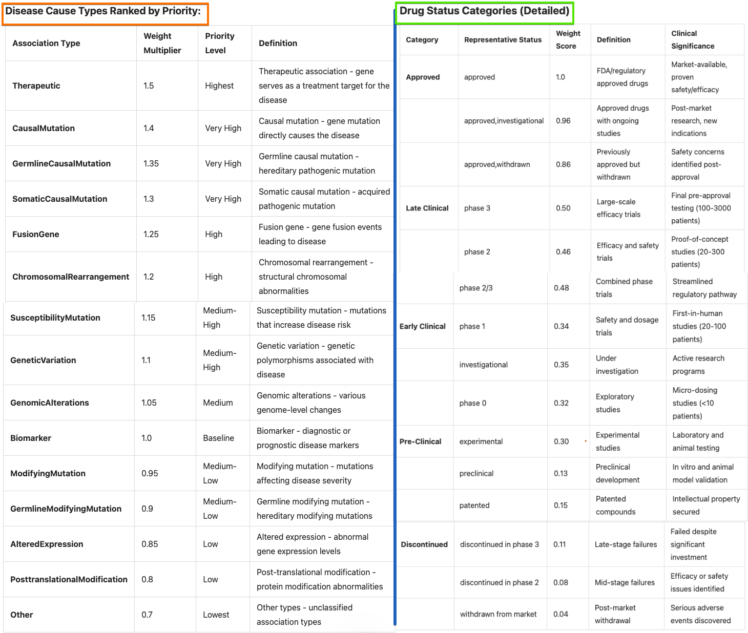
• Research Priority: Annotation-based priority label (Final Composite Score >= 0.7 ~ High Priority; Final Composite Score >= 0.4 ~ Medium Priority)
• Target Type: Disease-context Polycomb annotation category

Gene-Disease-Drug Network Visualization:

• Drug Nodes (Circle): Drug or compound annotations linked to query genes
• Meaning: Drug-gene records that may support follow-up research
• Central Gene Nodes (Square): User-selected query genes
• Meaning: Candidate Polycomb target records with disease or drug annotations
• Disease Nodes (Triangle): Disease annotations linked to query genes
• Meaning: Disease-context information from external resources

Identify predicted transcription-factor binding motifs within promoters of candidate Polycomb target genes. The module integrates JASPAR motif databases to analyse gene-motif relationships across human and mouse species. Motif results are promoter-level hypotheses and should not be interpreted as direct evidence of tissue-specific transcription-factor binding.

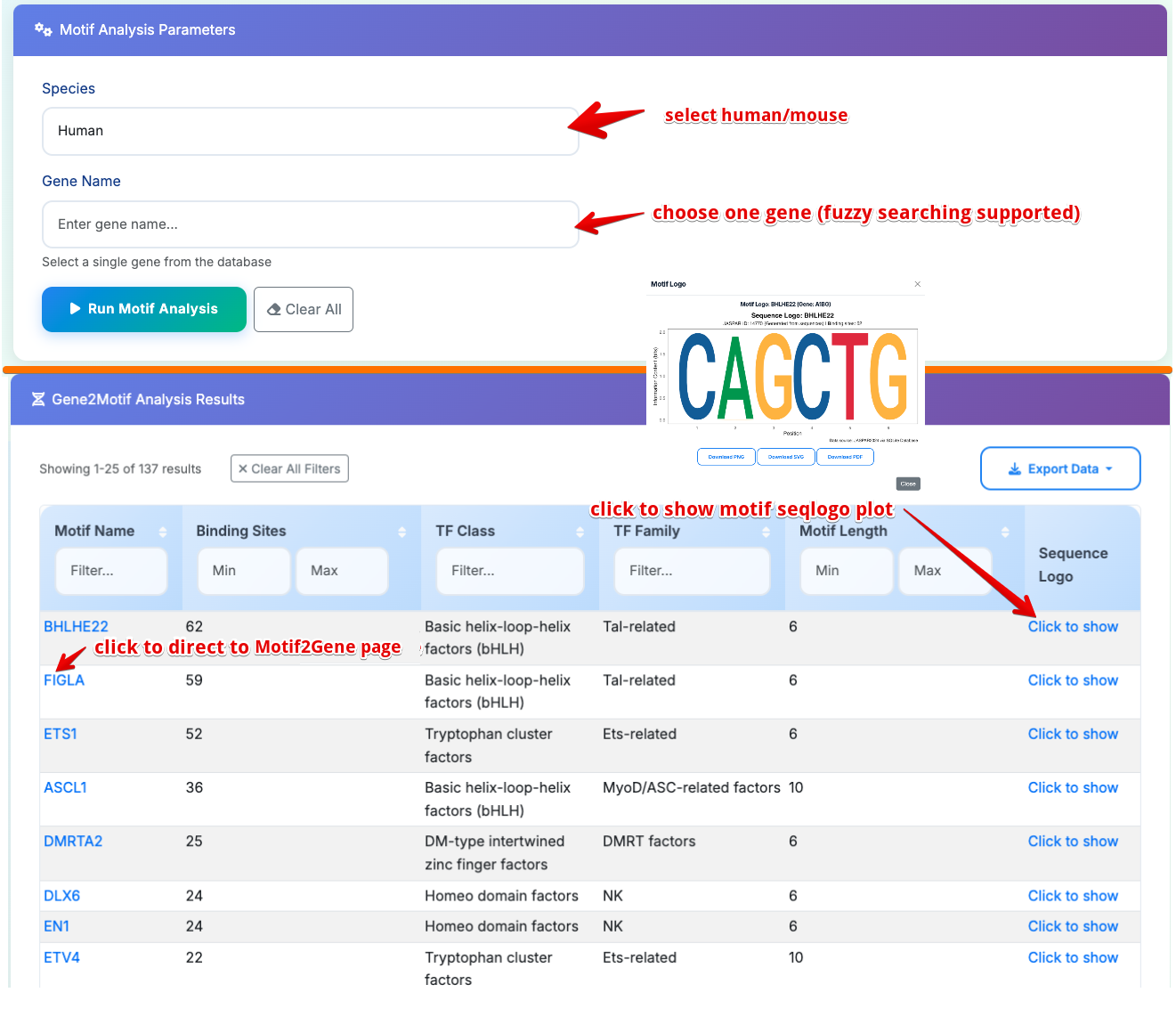
Sub-Module 1: Gene2Motif Analysis

Purpose: Find predicted transcription-factor binding motifs present in the promoter of a specific gene

Usage:

1. Select Species: Choose Human or Mouse from dropdown
2. Select Gene: Click dropdown to search and select one gene from database
3. Run Analysis: Click Run Motif Analysis to execute

Results Table Columns: - Motif Name: JASPAR motif identifier with cross-reference links - Binding Sites: Number of predicted motif matches in promoter sequence - TF Class: Transcription factor structural classification - TF Family: Transcription factor family grouping - Motif Length: Length of consensus binding sequence - Show Motif Logo: Sequence logo visualization

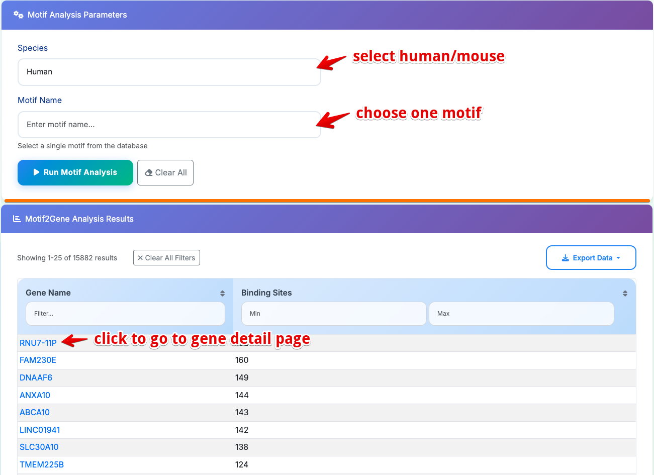
Sub-Module 2: Motif2Gene Analysis

Purpose: Find genes whose promoter sequences contain a selected predicted transcription-factor motif

Usage:

1. Select Species: Choose Human or Mouse from dropdown
2. Select Motif: Click dropdown to search and select motif from database
3. Run Analysis: Click Run Motif Analysis to execute

Results Table Columns:

• Gene Name: Gene symbol with direct links to gene details pages
• Binding Sites: Number of predicted motif matches

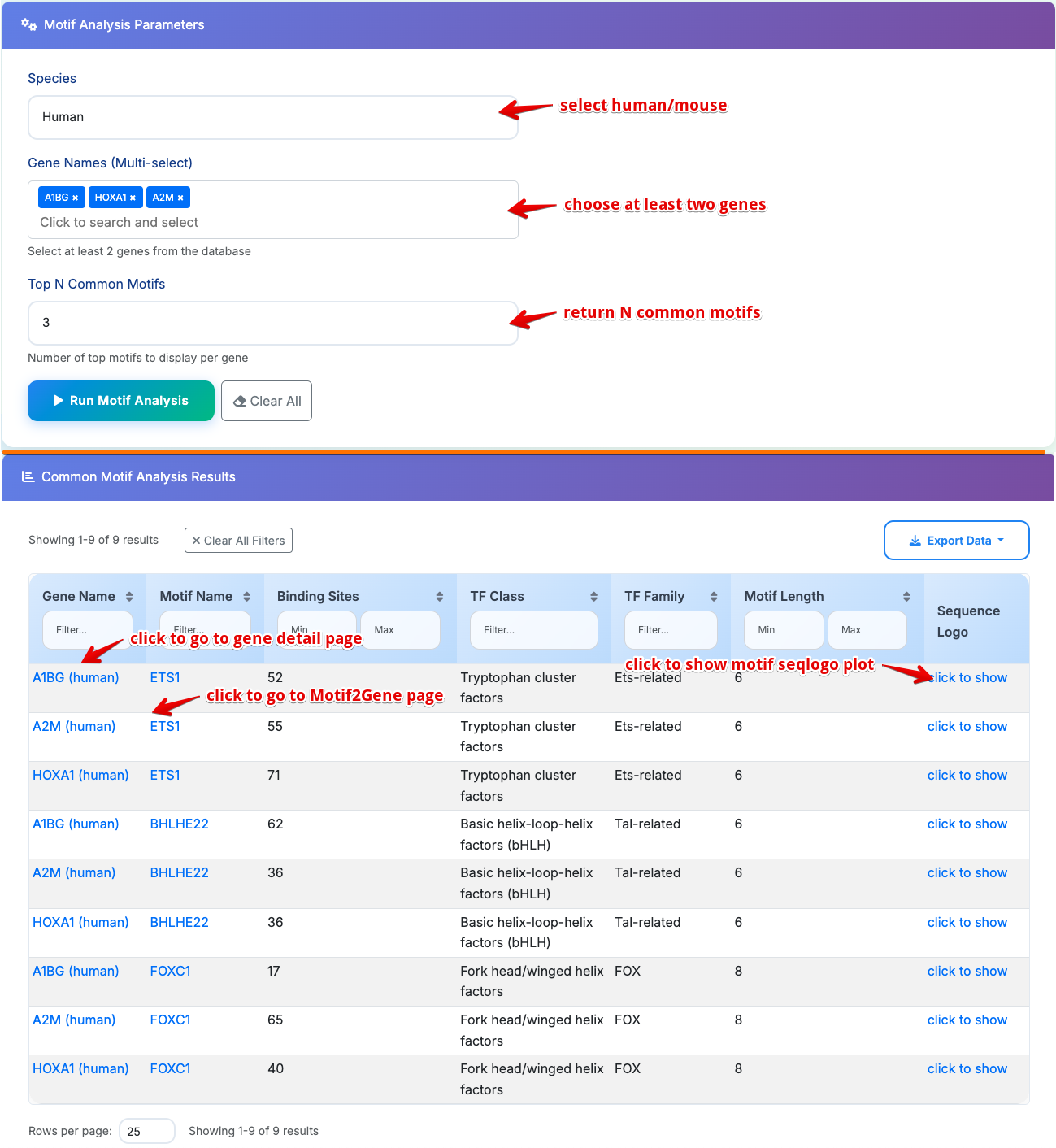
Sub-Module 3: Common Motif Analysis

Purpose: Identify predicted promoter motifs shared among multiple genes

Usage:

1. Select Species: Choose Human or Mouse from dropdown
2. Multi-Gene Selection: Click dropdown to select multiple genes (minimum 2 required) . Selected genes appear as tags with removal options; Supports fuzzy search for gene discovery
3. Set Parameters: Configure "Top N Common Motifs" (5-50, default: 10)
4. Run Analysis: Click Run Motif Analysis to execute

Results Table Columns:

• Gene Name: Gene symbol with species-specific links
• Motif Name: Shared motif identifier with cross-navigation to Motif2Gene
• Binding Sites: Number of predicted motif matches in each gene promoter
• TF Class: Transcription factor classification
• TF Family: Transcription factor family
• Motif Length: Consensus sequence length
• Show Motif Logo: Sequence logo visualization

PRIME provides direct access to three categories of precompiled, reusable data files without requiring users to rerun analyses.

Data Categories:

1. Candidate Polycomb Regulatory Target Records

• 8 datasets: Human/Mouse × Normal/Disease × All/High-confidence
• File sizes: 1.4MB - 49.4MB
• Content: Cross-species and condition-specific candidate Polycomb target records with PTS and confidence information

2. Disease-Related Target Annotations

• Single Excel file (453KB) with 4 sheets
• Content: Disease-context annotations and analysis outputs for candidate Polycomb target records

3. Literature Mining Results

• Single Excel file (768KB)
• Content: Systematically extracted Polycomb-related information from peer-reviewed literature

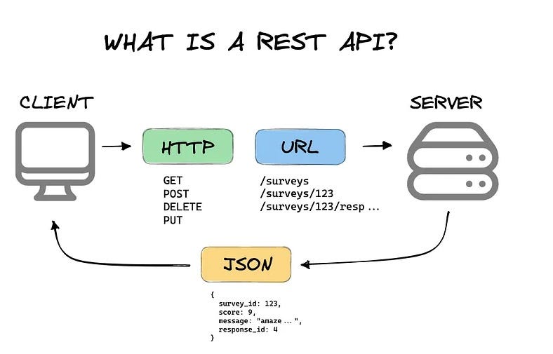
PRIME provides a comprehensive RESTful API for accessing all platform data and functionality programmatically. It is designed for researchers who want to build custom analysis pipelines or integrate PRIME data into larger workflows.

Base URL: https://primedb.org/api/

Gene Information APIs

• /api/gene/{gene_name}/info - Gene details and annotations
• /api/gene/{gene_name}/coordinates - Genomic coordinates for browser
• /api/gene/{gene_name}/external_db - External database links

Expression Data APIs

• /api/gene/{gene_name}/bodymap - PTS tissue-profile data
• /api/expression/{atlas}/{gene_name}/plot - Expression atlas plots (GTEx, TCGA, HPA, FANTOM5)

Search & Browse APIs

• POST /api/search/execute - Advanced search with filtering
• /api/gene_suggestions - Gene name autocomplete
• /api/browse/datasets - Dataset browsing with filters

Analysis APIs

• POST /api/analysis/comparison/run - Species/tissue/status comparisons
• POST /api/analysis/network/run - Regulatory network analysis
• POST /api/analysis/motif/run - Motif analysis (Gene2Motif, Motif2Gene, Common)

Download APIs

• /api/download/polycomb/{dataset}/{format} - Precompiled data files
• POST /api/search/download - Custom search result exports

Response Format:

All APIs return JSON with standardised error handling:

• HTTP 200: Success
• HTTP 400: Invalid parameters
• HTTP 404: Resource not found

How is PRIME built?

Backend Framework:

• Flask web framework with Python for page rendering, query handling and user-facing modules
• Structured API endpoints for programmatic access to gene information, search results, visualisation data and analysis outputs
• Relational database tables and precomputed evidence records for efficient retrieval of COMPASS-derived scores and annotation layers

Data Processing:

• Python-R hybrid architecture: Python handles database operations and dynamic interactive visualisations, while R scripts generate selected statistical outputs and publication-style plots
• Precomputed COMPASS outputs: PTS values, confidence tiers and primary evidence summaries are calculated before database loading
• Specialised data stores for modules such as motif analysis, expression atlases, literature-derived records and genome-track visualisation
• BigWig file format for efficient genomic track storage and IGV.js integration

Frontend Technologies:

• Bootstrap 5 for responsive design and user interface components
• IGV.js for interactive genome-browser functionality
• Plotly.js for dynamic data visualisations and charts
• Custom JavaScript for user interactions and API communication

Scientific Integration:

• Multi-omics evidence integration from H3K27me3 ChIP-seq, PcG perturbation RNA-seq and curated literature-derived records
• External annotation layers including GTEx, TCGA, HPA and FANTOM5 for expression and protein-context interpretation
• Disease, drug, network and motif annotations for downstream evidence inspection and hypothesis generation

Deployment:

• Docker containerisation for consistent deployment across environments
• Gunicorn WSGI server for production deployment within containers
• Reverse-proxy support for stable web access
• Environment-based configuration for flexible deployment

This architecture keeps COMPASS scoring outputs stable and traceable while allowing PRIME to provide search, visualisation, comparison, annotation and download functions through a user-friendly web interface.

Which species are supported?

PRIME currently supports Human (Homo sapiens) and Mouse (Mus musculus), the two species with the broadest public PcG-related RNA-seq and H3K27me3 ChIP-seq evidence coverage.

How are confidence levels determined?

• Adaptive tissue-specific thresholds: Different percentile cutoffs adjusted by tissue size to ensure comparable results
• Integrated multi-omics evidence: Combined H3K27me3 ChIP-seq chromatin-state evidence and PcG perturbation RNA-seq response evidence
• Hierarchical scoring system: Three-tier classification based on final composite scores

Three levels:

• High: Strongest integrated evidence for PcG-associated prioritisation (80-90th percentile, depending on tissue size: ≥10,000 genes use 90%, 5,000-10,000 use 85%, <5,000 use 80%)
• Medium: Moderate integrated evidence (>50th percentile threshold)
• Low: Weak, incomplete or no clear evidence in the available data

Why are some search results empty?

Because there may be no corresponding evidence entry, no sufficient data coverage or no result passing the selected filters for that gene/tissue combination.

Why might pages load slowly?

Some modules load large precomputed tables, genome tracks or interactive visualisations. Complex queries may take 30-60 seconds to complete.

Can I download all data at once?

Yes. Use the Download page to get precompiled data files, or export custom results from Search and Browse pages.

How to cite PRIME?

Please cite PRIME in your publications. Citation information will be provided upon database publication.